PyIT2FLS

PyIT2FLS is providing a set of tools for fast and easy modeling of Interval Type 2 Fuzzy Sets (IT2FS) and Systems (IT2FLS). There are two main classes in this toolkit, named IT2FS and IT2FLS. The first one is for defining IT2FSs and the latter is for defining IT2FLSs. There are many functions defined in PyIT2FLS for utilizing these two classes, which would be introduced in the following.

IT2FS

In this section, we are going to see how IT2FSs can be defined using the IT2FS class. An IT2FS is defined by its Lower Membership Function (LMF) and Upper Membership Function (UMF). So first we need to know functions, which can be used as LMFs and UMFs. The list of membership functions provided with the PyIT2FLS is presented below:

List of membership functions that can be used as LMF and UMF functions

Membership function	Description	List of parameters
zero_mf	All zero membership function	None
singleton_mf	Singleton membership function	Singleton’s center and height
const_mf	Constant membership function	Constant membership function’s height
tri_mf	Triangular membership function	The left end, the center, the right end, and the height of the triangular membership function
ltri_mf	Left triangular membership function	The right end, the center, and the height of the triangular membership function
rtri_mf	Right triangular membership function	The left end, the center, and the height of the triangular membership function
trapezoid_mf	Trapezoidal membership function	The left end, the left center, the right center, the right end, and the height of the trapezoidal membership function
gaussian_mf	Gaussian membership function	The center, the standard deviation, and the height of the gaussian membership function
gauss_uncert_mean_umf	Gaussian with uncertain mean UMF	The lower limit of mean, the upper limit of mean, the standard deviation, and the height of the gaussian membership function
gauss_uncert_mean_lmf	Gaussian with uncertain mean LMF	The lower limit of mean, the upper limit of mean, the standard deviation, and the height of the gaussian membership function
gauss_uncert_std_umf	Gaussian with uncertain standard deviation UMF	The center, the lower limit of std., the upper limit of std., and the height of the gaussian membership function
gauss_uncert_std_lmf	Gaussian with uncertain standard deviation LMF	The center, the lower limit of std., the upper limit of std., and the height of the gaussian membership function

It must be noticed that the parameters of the introduced functions are passed as a list with items mentioned, respectively.

Creating an IT2FS

The constructor function of the IT2FS class has six parameters, listed as below:

domain: The universe of discourse of the interval type 2 fuzzy set
umf: The UMF of the interval type 2 fuzzy set
umf_params: The parameters of the UMF function
lmf: The LMF of the interval type 2 fuzzy set
lmf_params: The parameters of the LMF function
check_set: Boolean with default False value. If it is set as True then while the set is creating the condition of LMF(x)<=UMF(x) is checked for each x in domain.

Example 1

The first example demonstrates how to create an IT2FS with trapezoid LMF and triangular UMF functions:

from pyit2fls import IT2FS, trapezoid_mf, tri_mf
from numpy import linspace

mySet = IT2FS(linspace(0., 1., 100), 
              trapezoid_mf, [0, 0.4, 0.6, 1., 1.], 
              tri_mf, [0.25, 0.5, 0.75, 0.6])

In the first line, the IT2FS class and trapezoid and triangular membership functions are imported from the toolkit. Also in the second line, from the NumPy, the linspace is imported for creating the domain of the set. Then, using the IT2FS, the interval type 2 fuzzy set, named mySet, is created.

Creating common gaussian interval type 2 fuzzy sets

Most of the time, the gaussian interval type 2 fuzzy sets are preferred in applications. There are two types of gaussian sets, gaussian interval type 2 fuzzy sets with uncertain mean value and gaussian interval type 2 fuzzy sets with uncertain standard deviation value. To define sets of these types, it is not needed to define LMF and UMF functions and specify their parameters. There are two functions for defining these sets fastly and easily, IT2FS_Gaussian_UncertMean and IT2FS_Gaussian_UncertStd. Each of these functions has two input parameters, named domain and params. The domain input is the universe of discourse, in which the set is defined on it. The params input for the IT2FS_Gaussian_UncertMean function is a list consisting of the mean center, the mean spread, the standard deviation, and the height of the set. And for the IT2FS_Gaussian_UncertStd function, it is a list consisting of the mean, the standard deviation center, the standard deviation spread, and the height of the set.

Plotting the IT2FSs

To plot an IT2FS, the plot function from the IT2FS class can be used. This function has three input parameters with None default value, named title, legend_text, and filename. If the title and legend_text parameters are set, the plot would be done using them. And if the filename is set, the output figure would be saved as a pdf file with the specified name. Example 1 can be completed by plotting the output set using the plot function as below:

from pyit2fls import IT2FS, trapezoid_mf, tri_mf
from numpy import linspace

mySet = IT2FS(linspace(0., 1., 100), 
              trapezoid_mf, [0, 0.4, 0.6, 1., 1.], 
              tri_mf, [0.25, 0.5, 0.75, 0.6])
mySet.plot(filename="mySet")

Plotting multiple IT2FSs together

If there are many sets which we would like to plot them together, we can use the IT2FS_plot function from PyIT2FLS. The inputs of this function, after an arbitrary number of IT2FSs, are like plot function. It means that three title, legend_text, and filename parameters with the None default value. In the second example below, it is shown how to use the IT2FS_plot function for plotting three IT2FSs.

Example 2

The second example demonstrates how to define gaussian IT2FSs and plot them together.

from pyit2fls import IT2FS_Gaussian_UncertMean, IT2FS_plot, meet, join, min_t_norm, max_s_norm
from numpy import linspace

domain = linspace(0., 1., 100)
A = IT2FS_Gaussian_UncertMean(domain, [0., 0.1, 0.1, 1.])
B = IT2FS_Gaussian_UncertMean(domain, [0.33, 0.1, 0.1, 1.])
C = IT2FS_Gaussian_UncertMean(domain, [0.66, 0.1, 0.1, 1.])
IT2FS_plot(A, B, C, title="", legends=["Small","Medium","Large"], filename="multiSet")

T-norms and S-norms

In the PyIT2FLS, there are two T-norms and an S-norm by default, however, new ones can be defined by the users. Any function that theoretically meets the requirements of T-norm (or S-norm) and is defined as the following can be used as a T-norm (or S-norm). The function that is going to be used as a T-norm (or S-norm) must have two inputs. These inputs would be NumPy (n,) shaped arrays (or single float number). The output must be also of the type NumPy (n,) shaped array (or single float number). The function must be compatible with these two input/output types. The functions from the PyIT2FLS dedicated to T-norms and S-norms are as below:

min_t_norm: Minimum T-norm
product_t_norm: Product T-norm
max_s_norm: Maximum S-norm

Meet and join operators

Two essential operators in Interval Type 2 Fuzzy Logic, are the meet and join operators. These operators are defined in PyIY2FLS as two functions meet and join. Both functions have four inputs. For these functions, the first three inputs are common, the universe of discourse, the first IT2FS, and the second IT2FS. The 4th input of the meet function is the desired T-norm function, and for the join function, it is the desired S-norm function.

Example 3

Completing the second example, the meet of the sets A and B, and join of the sets B and C are calculated:

from pyit2fls import IT2FS_Gaussian_UncertMean, IT2FS_plot, meet, join, min_t_norm, max_s_norm
from numpy import linspace

domain = linspace(0., 1., 100)
A = IT2FS_Gaussian_UncertMean(domain, [0., 0.1, 0.1, 1.])
B = IT2FS_Gaussian_UncertMean(domain, [0.33, 0.1, 0.1, 1.])
C = IT2FS_Gaussian_UncertMean(domain, [0.66, 0.1, 0.1, 1.])
IT2FS_plot(A, B, C, title="", legends=["Small","Medium","Large"], filename="multiSet")

AB = meet(domain, A, B, min_t_norm)
AB.plot(filename="meet")

BC = join(domain, B, C, max_s_norm)
BC.plot(filename="join")

Type reduction algorithms

The type reduction plays a key role in achieving crisp values from Type 2 Fuzzy Sets. The type reduction algorithms, which are implemented in the PyIT2FLS, are listed as the table below.

Type reduction algorithm function	Description
KM_algorithm	Karnik-Mendel algorithm
EKM_algorithm	Enhanced Karnik-Mendel algorithm
WEKM_algorithm	Weighted enhanced Karnik-Mendel algorithm
TWEKM_algorithm	Trapezoid weighted enhanced Karnik-Mendel algorithm
EIASC_algorithm	Enhanced Iterative Algorithm with Stopping Condition
WM_algorithm	Wu-Mendel algorithm
BMM_algorithm	Begian-Melek-Mendel algorithm
LBMM_algorithm	Li-Begian-Melek-Mendel algorithm
NT_algorithm	Nie-Tan algorithm

IT2FLS

In this section, along with introducing the IT2FLS class, a simple Interval Type 2 Fuzzy Logic Controller (IT2FLC) is designed for stabilizing the inverted pendulum system. The equations of the inverted pendulum system are adapted from the book A Course in Fuzzy Systems and Control by Li-Xin Wang, and are represented below:

$\dot{x}_{1} = x_{2}$

$\dot{x}_{2} = \frac{gsinx_{1}-\frac{mlx_{2}^{2}cosx_{1}sinx_{1}}{m_{c}+m}}{l\left(\frac{4}{3}-\frac{mcos^{2}x_{1}}{m_{c}+m}\right)}+\frac{\frac{cosx_{1}}{m_{c}+m}}{l\left(\frac{4}{3}-\frac{mcos^{2}x_{1}}{m_{c}+m}\right)}u$

For creating an IT2FLS using the PyIT2FLS library, the IT2FLS class should be used. The constructor function of this class doesn’t need any parameter. The code below creates an IT2FLS:

from pyit2fls import IT2FLS
it2fls = IT2FLS()

The next step for defining and using an IT2FLS is to define its inputs and outputs. The function add_input_variable adds input variables to the system. The only input for this function is the name of the input. The input names are added to a list in the IT2FLS class, named inputs. Also, the function add_output_variable add output variables to the system. This function, like the previous one, has just a single input, the name of the output. In our controller design example, the only control signal is designed based on state feedback. So the fuzzy controller must have two inputs. Let’s define the input and outputs for the IT2FLS:

it2fls.add_input_variable("x1")
it2fls.add_input_variable("x2")
it2fls.add_output_variable("O")

Now it is time to define If-Then rules. The function add_rule is used for adding new rules to the system. These rules are added to a list in IT2FLS class, named rules. This function has two inputs which are of list type. The first input is a list of tuples, in which the first element of each tuple is an input name and the second element is an IT2FS. Also, the second output is a list of tuples, in which the first element is an output name and the second element is an IT2FS. Let’s consider the rule base of our IT2FLC as below:

IF x1 is N AND x2 is N THEN O is P
IF x1 is N AND x2 is P THEN O is Z
IF x1 is P AND x2 is N THEN O is Z
IF x1 is P AND x2 is P THEN O is N

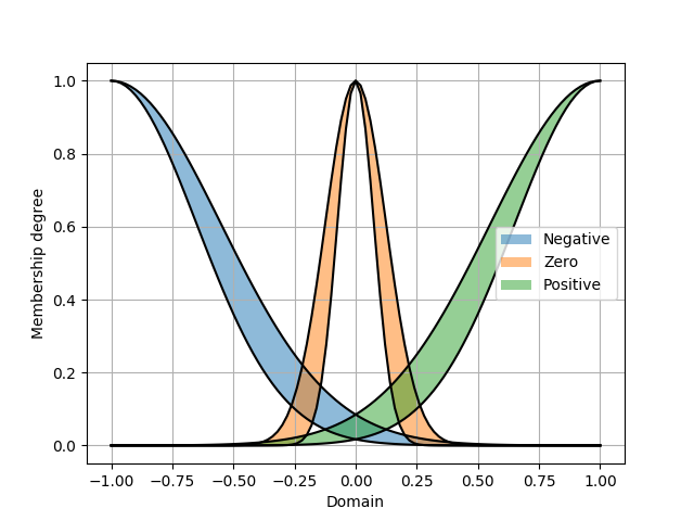
In these rules, N, Z, and P are fuzzy sets defined in the interval [-1, 1]. N stands for Negative, Z for Zero, and P for Positive. Before adding rules to our IT2FLC, let’s define these sets as Gaussian IT2FSs with uncertain standard deviation value and plot them:

from numpy import  linspace
from pyit2fls import IT2FS_Gaussian_UncertStd, IT2FS_plot

domain = linspace(-1., 1., 101)
N = IT2FS_Gaussian_UncertStd(domain, [-1., 0.4, 0.1, 1.])
Z = IT2FS_Gaussian_UncertStd(domain, [0., 0.1, 0.05, 1.])
P = IT2FS_Gaussian_UncertStd(domain, [1., 0.4, 0.1, 1.])
IT2FS_plot(N, Z, P, 
           legends=["Negative", "Zero", "Positive"])

The sets would be as below:

The IT2FSs are ready now, so we can define our rule base as below, using the function add_rule:

it2fls.add_rule([("x1", N), ("x2", N)], [("O", P)])
it2fls.add_rule([("x1", N), ("x2", P)], [("O", Z)])
it2fls.add_rule([("x1", P), ("x2", N)], [("O", Z)])
it2fls.add_rule([("x1", P), ("x2", P)], [("O", N)])

Let’s compare a rule and the corresponding code for clarifying the process of adding rules to the rule base of the system. The second rule is considered as:

IF x1 is N AND x2 is P THEN O is Z

And the code dedicated to define the rule is:

it2fls.add_rule([("x1", N), ("x2", P)], [("O", Z)])

In the second rule, the input x1 is checked with the set N and the input x2 is checked with the set P. The first input of the function add_rule, which defines the antecedent part of the rule, must consist of two tuples. One for input x1 and the other for input x2. As it is said, the first element of the tuples must be the input name and the second element, the corresponding set. So the first tuple is (“x1”, N) and the second one is (“x2”, P). Furthermore, the second input of the function add_rule, which defines the consequent part of the rule, must consist of a tuple. This is because we have only one output in our IT2FLS. So the first element of the tuple, which indicates the output name, must be “O”. And the second element of the tuple, which is the corresponded fuzzy set, must be Z. Finally, the tuple would be as (“O”, Z).

The IT2FLC is now ready for evaluating the inputs. The function evaluate defined in the IT2FLS class should be used for this purpose. This function has eight inputs, which four of them have default values but the other four must be given by the user always. The inputs of this function are inputs, T-norm, S-norm, universe of discourse, method, method parameters (method_params), algorithm, and algorithm parameters(algorithm_params). The first input is of type dictionary, which its keys are the input names and its values are corresponding values of inputs. T-norm, S-norm, type reduction algorithm and its parameters are discussed before. Type reduction algorithm by default is set to “EIASC” and its parameters (algorithm_params) is set to None. There are many methods to evaluate an IT2FLS which are listed in the table below:

IT2FLS evaluation methods	Description
Centroid	Centroid method
CoSet	Center of sets method
CoSum	Center of sum method
Height	Height method
ModiHe	Modified height method

The method input of the evaluate function must be one of the methods introduced above. Some of these methods may need some parameters which can be passed using the method_params input of the evaluate function. Detailed information about these methods and their parameters are accessible from docstrings. It must be noticed that the Centroid method is more common in control applications.

Coming back to our inverted pendulum control system, the function for evaluating the control signal can be written as below:

from pyit2fls import product_t_norm, max_s_norm

def u_fuzzy(X, t):
    x1 = max(-1., min(1., X[0]))
    x2 = max(-1., min(1., X[1]))
    c, TR = it2fls.evaluate({"x1":x1, "x2":x2},
                    product_t_norm, max_s_norm, domain, method="Centroid", 
                    algorithm="EKM")
    o = (TR["O"][0] + TR["O"][1]) / 2
    return 20 * o

In the code above the variables X[0] and X[1] are our system’s state variables. Since the universe of discourse is defined in the interval [-1,1], so the state variables as inputs of the IT2FLC must be clipped into this interval. The variables x1 and x2 are clipped version of state space variables. After that, the system is evaluated for the inputs x1 and x2. As it is mentioned in the docstrings, when we are using the Centroid method, the outputs of the evaluate function are the resultant IT2FS and type reduced version of it. The type reduced output is store in the TR, which is defuzzified and stored in the variable o. The final control signal is scaled version of the output of the IT2FLS. The codes for the inverted pendulum control example can be summed up as below with some plots:

import matplotlib.pyplot as plt
from pyit2fls import IT2FS_Gaussian_UncertStd, IT2FLS, \
                     min_t_norm, product_t_norm, max_s_norm, IT2FS_plot
from numpy import  array, linspace
from numpy import cos as c, sin as s
from scipy.integrate import odeint


g = 9.8
mc = 1.
m = 0.1
l = 0.5

def dynamic(X, t, u):
    x1 = X[0]
    x2 = X[1]
    x1_dot = x2
    x2_dot = (g * s(x1) - 
              m * l * x2 ** 2 * c(x1) * s(x1) / (mc + m)) / \
        (l * (4./3. - m * c(x1) ** 2 / (mc + m))) + \
        u(X, t) * (c(x1) / (m + mc)) / (l * (4./3. - m * c(x1) ** 2 / (mc + m)))
    return array([x1_dot, 
                  x2_dot])


if __name__ == "__main__":
    
    domain = linspace(-1., 1., 101)
    N = IT2FS_Gaussian_UncertStd(domain, [-1., 0.4, 0.1, 1.])
    Z = IT2FS_Gaussian_UncertStd(domain, [0., 0.1, 0.05, 1.])
    P = IT2FS_Gaussian_UncertStd(domain, [1., 0.4, 0.1, 1.])
    IT2FS_plot(N, Z, P, 
               legends=["Negative", "Zero", "Positive"])
    
    it2fls = IT2FLS()
    it2fls.add_input_variable("x1")
    it2fls.add_input_variable("x2")
    it2fls.add_output_variable("O")
    
    it2fls.add_rule([("x1", N), ("x2", N)], [("O", P)])
    it2fls.add_rule([("x1", N), ("x2", P)], [("O", Z)])
    it2fls.add_rule([("x1", P), ("x2", N)], [("O", Z)])
    it2fls.add_rule([("x1", P), ("x2", P)], [("O", N)])

    def u_fuzzy(X, t):
        x1 = max(-1., min(1., X[0]))
        x2 = max(-1., min(1., X[1]))
        c, TR = it2fls.evaluate({"x1":x1, "x2":x2},
                        product_t_norm, max_s_norm, domain, method="Centroid", 
                        algorithm="EKM")
        o = (TR["O"][0] + TR["O"][1]) / 2
        return 40 * o
    
    def u_zero(X, t):
        return 0
        
    
    X0 = [-2., 0.]
    t = linspace(0.0, 10.0, 1000)
    X = odeint(dynamic, X0, t, args=(u_zero, ))
    plt.figure()
    plt.plot(t, X[:, 0], label=r"$x_{1}$")
    plt.plot(t, X[:, 1], label=r"$x_{2}$")
    plt.xlabel("t (s)")
    plt.legend()
    plt.grid(True)
    plt.show()
    
    X = odeint(dynamic, X0, t, args=(u_fuzzy, ))
    plt.figure()
    plt.plot(t, X[:, 0], label=r"$x_{1}$")
    plt.plot(t, X[:, 1], label=r"$x_{2}$")
    plt.xlabel("t (s)")
    plt.legend()
    plt.grid(True)
    plt.show()
    
    u = []
    for x, tt in zip(X, t):
        u.append(u_fuzzy(x, tt))
    u = array(u)
    plt.figure()
    plt.plot(t, u, label=r"Fuzzy Controller")
    plt.xlabel("t (s)")
    plt.legend()
    plt.grid(True)
    plt.show()

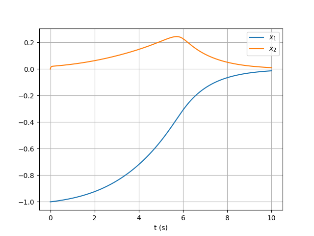
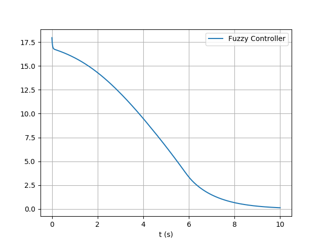
The output of the simulation is demonstrated in the figures below. The first figure is state space variables of the system and the second figure is the generated fuzzy control signal over time.